1
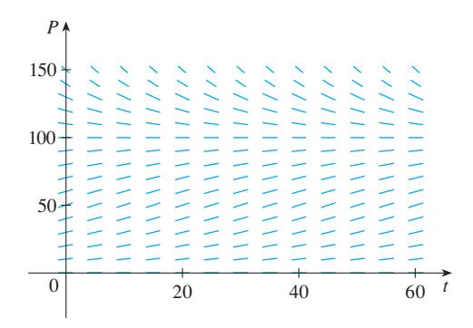
A population grows according to the given logistic equation, where \(t\) is measured in weeks.
\( \dfrac{d P}{d t} = 0.04 P \left(1 - \dfrac{P}{1200}\right), \quad P(0) = 60 \)
(a) What is the carrying capacity? What is the value of \(k\)?
(b) Write the solution of the equation.
(c) What is the population after 10 weeks?
Enter your answer directly below each part above.
Click to select photo