1
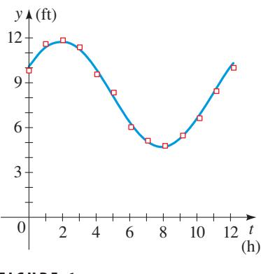
A set of data is given. (a) Make a scatter plot of the data. (b) Find a cosine function of the form \(y = a \cos(\omega (t - c)) + b\) that models the data, as in Example 1. (c) Graph the function you found in part (b) together with the scatter plot. How well does the curve fit the data? (d) Use a graphing calculator to find the sine function that best fits the data, as in Example 2. (e) Compare the functions you found in parts (b) and (d). [Use the reduction formula \(\sin u = \cos\left(u - \dfrac{\pi}{2}\right)\).] Data: \(t\) = 0, 2, 4, 6, 8, 10, 12, 14; \(y\) = 2.1, 1.1, -0.8, -2.1, -1.3, 0.6, 1.9, 1.5.
Click to select photo