1
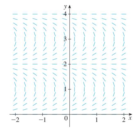
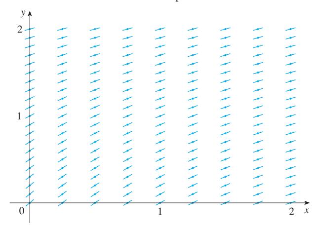
A direction field for the differential equation \(y' = x \cos \pi y\) is shown.
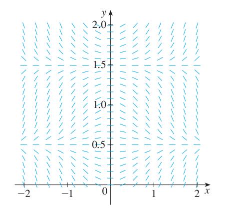
(a) Sketch the graphs of the solutions that satisfy the given initial conditions.
(i) \(y(0) = 0\) \(\quad\) (ii) \(y(0) = 0.5\) \(\quad\) (iii) \(y(0) = 1\) \(\quad\) (iv) \(y(0) = 1.6\)
(b) Find all the equilibrium solutions.
Enter your answer directly below each part above.
Click to select photo